Economic Value Mapping service specifications

Find EVM service tutorial here.
Service Description
The Economic Value Mapping (EVM) service focuses on exploiting multisource geospatial, statistical and economic information to accurately map the economic value of assets. The products of this service can support impact and risk assessment when properly overlaid with vulnerability and hazard information, thereby aiding in mitigation strategies and decision-making.
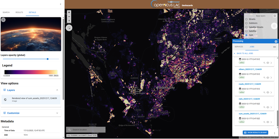
In terms of geophysical products, the EVM service generates on demand a land use/land cover map with each pixel depicting specific asset category quantified in USD/m2, over the Area of Interest selected by the user.
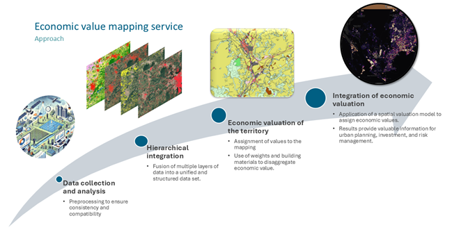
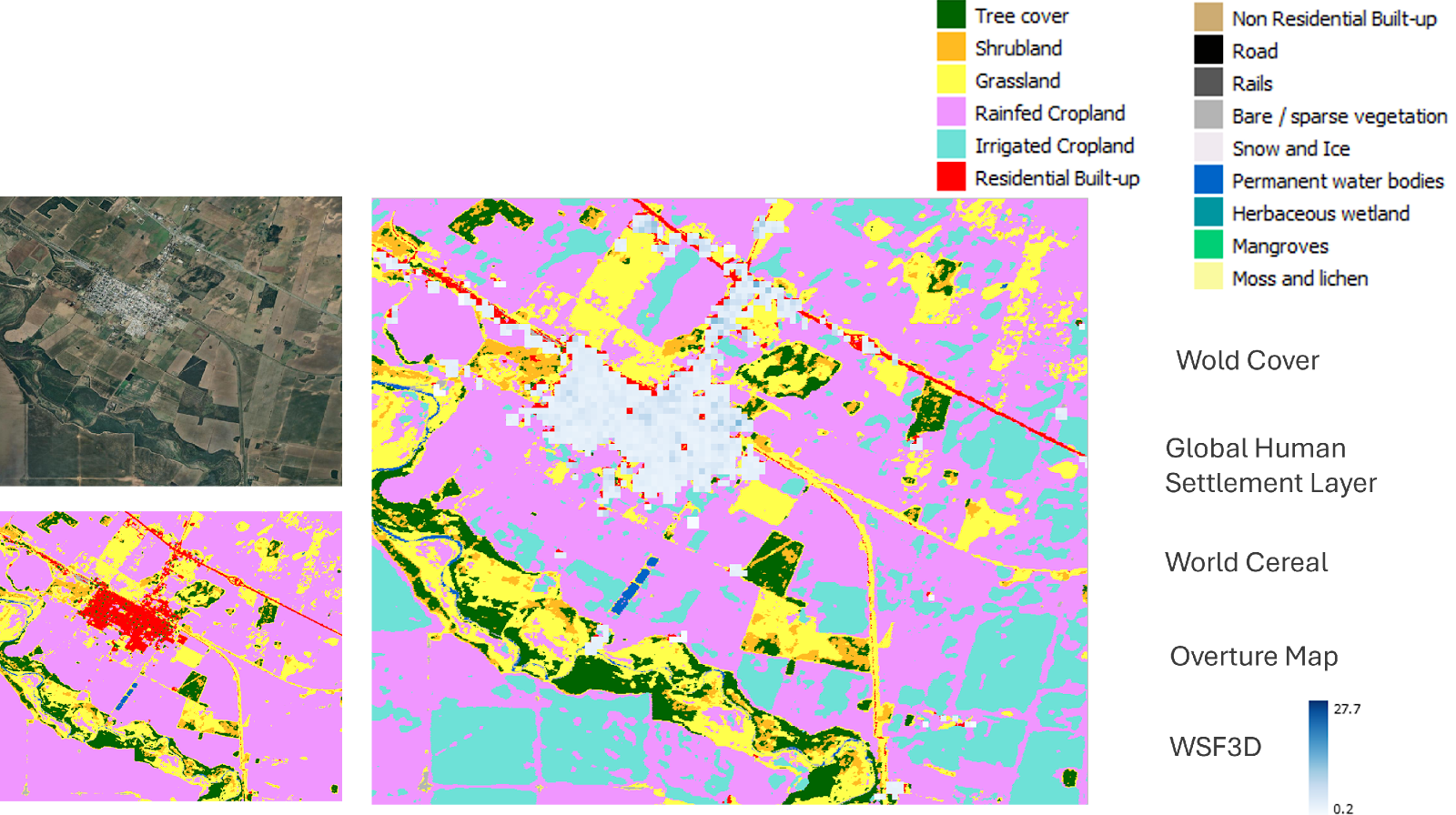
This service follows a hierarchical approach to aggregate multiple geospatial data sources into a unified structured set. Next, new features are integrated to enhance spatial representation such as country boundaries, road networks, building heights and population. Finally, the economic values are assigned through a spatial valuation model based on statistical values disaggregation and weights application.
Economic Basis of the service
The EVM service is based on geospatial data combined with economic values representing the monetary exposure of physical assets. These values are expressed as the total accumulated cost (in USD) for each asset category, either at the national level (default) or customized by the user.
The service relies on two types of economic data sources:
-
Default values: Predefined estimates of asset values at the national level
-
User provided values: Custom inputs that can either: -Replace the national defaults for the entire country, or
- Specify localized values for the selected AOI
These asset values represent the economic exposure of different components. The categories include:
-
Private Housing : Residential buildings such as homes and apartments.
-
Household Content : Furniture, appliances, and household goods inside homes.
-
Industrial Buildings and Equipment : Factories, warehouses, and machinery.
-
Services and Trade Buildings and Equipment : Offices, schools, hospitals, shops, and related equipment.
-
Agricultural Buildings and Equipment : Farm structures and machinery.
-
Industrial Inventories : Goods and materials stored by manufacturing industries.
-
Services and Trade Inventories : Stock held by service providers and trade businesses.
-
Vehicles : Cars, trucks, and other motor vehicles.
-
Livestock : Animals used for meat, dairy, and related products.
-
Agricultural Stocks: Stored crops and agricultural products.
-
Roads: The existing road network.
-
Railways: The railway network.
-
Others (Green Spaces, Wetlands, Forests): Natural areas and forest resources.
Warning
DISCLAIMER: The default values for Private Housing, Industrial Buildings and Equipment, and Services and Trade Buildings and Equipment are derived from the Global Exposure Model (GEM), published by the GEM Foundation under the Creative Commons BY-NC-SA 4.0 license. Original data © GEM Foundation. For details on the license, visit: LICENSE. These values are used as input in the service to calculate exposure by area of interest and pixel type. No endorsement by GEM is implied.
Workflow
The schema shown in Figure 3 describes the execution scheme of the EVM service.
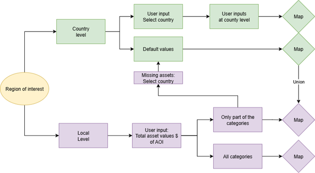
The execution scheme comprises the next steps:
-
Initial Decision: Before accessing the workspace, the user knows whether he/she will use default economic values or provide custom values (either at national or AOI level).
-
AOI selection: The user selects the Area of Interest on the map interface
-
Data Input:
- For national-level custom values, the user enters totals for one or more asset categories.
- For AOI-level custom values, the user provides complete or partial data for the selected area. If partial data is provided, the system retrieves missing values from the national dataset and adjusts them proportionally.
-
Map generation: The service integrates geospatial and economic data to produce maps showing economic exposure for each asset category.
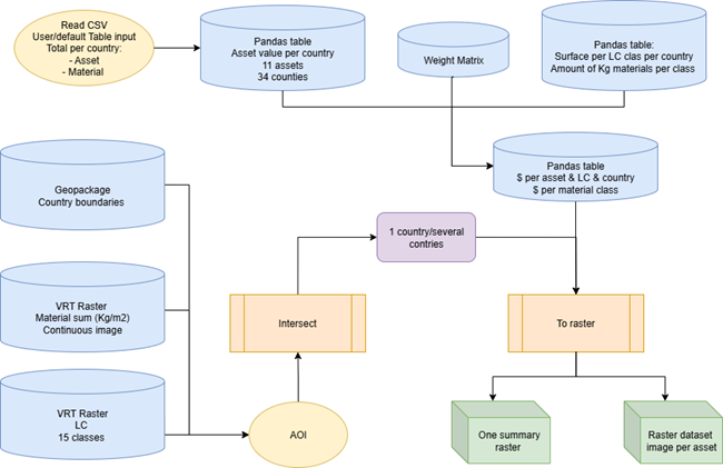
On the other hand, Figure 4 depicts the EVM workflow to transform user inputs and geospatial data into economic exposure maps. It consists into three main components:
Geospatial Data preparation
-
Inputs:
- Country boundaries (Geopackage format)
- Land cover raster (VRT) with 15 classes
- Material sum raster (VRT) representing accumulated material weight (kg/m2)
-
Process:
- The AOI selected by the user is intersected with these layers to clip the spatial data to the analysis extent.
- This step ensures that only relevant geospatial features are processed for valuation
Economic Data Processing
- Inputs:
- CSV file containing either default or user-provided economic values per country, including asset categories and material classes.
- Process:
- Build Pandas tables for asset values per country and for surface/material distribution per land cover class.
- Apply a weight matrix to link land cover classes with asset and material values.
- Compute monetary values ($) per asset and per material class for each country or AOI.
- Purpose:
- This step translates raw economic data into structured tables ready for spatial integration.
Integration and Map Production
- Process:
- Combine geospatial layers and economic tables for one or several countries.
- Convert results into raster outputs:
- One summary raster aggregating total economic exposure
- Raster dataset per asset category, providing detailed spatial distribution of values in USD/m2.
- Outputs:
- Georeferenced maps that can be used for impact and risk assessment when combined with hazard and vulnerability layers.
Inputs
The EVM service requires two types of inputs:
Dynamic Inputs (User Parameters)
Provided through the service form:
-
Area of Interest (AOI): Polygon defining the spatial extent of the analysis.
-
Country Code: ISO code identifying the country (e.g. GUY for Guyana).
-
Economic Values:
-
Default values: Predefined national-level totals for each asset category.
-
Custom values: User-provided totals for one or more asset categories.
-
-
Mode of Execution: Indicates whether custom values apply at national level or AOI level.
These parameters control the valuation process and determine how economic data is applied to the selected AOI.
For more information check the service tutorial.
Static Geospatial Inputs
Global datasets used for spatial allocation and weighting (not editable by the user):
| Data Type | Name | Update Year | Resolution | Definition, content |
|---|---|---|---|---|
| Base Land Cover | WorldCover | 2021 | 10 m | Main map, 8 classes |
| Built-Up Area | GHSL | 2018 | 10 m | Global layer of human settlement, 2 classes |
| Material Stock | WSF GlobMS | 2024 | 90 m | Global layer for quantification of building material stocks (concrete, steel, wood and bricks) |
| Crops Area | World Cereal | 2021 | 10 m | Global layers of Irrigated and non irrigated crop |
| Infrastructures | Overture Maps | 2022 | Vector file | Land use maps, road, building footprints, railways |
| Assets | Content | Type |
|---|---|---|
| Immobile | Buildings and equipment | Residential, industrial, agricultural |
| Mobile | Production, content | Industrial production, services and trade, household content |
Weighting Factors
The service applies fixed weighting factors to distribute economic values across land cover classes. These weights are predefined and cannot be modified by the user. They ensure that each asset category is spatially allocated according to land use and infrastructure patterns.
-
Industrial Building and Equipment:
- 20% in Built-up Residential
- 80% in Built-up Non-Residential
-
Services and Trade Building and Equipment
- 20% in Built-up Residential
- 80% in Built-up Non-Residential
-
Agricultural Building and Equipment
- 20% in Rainfed Croplands
- 60% in Irrigated Croplands
- 20% in Built-up Non-Residential
-
Industrial Inventories
- 20% in Built-up Residential
- 80% in Built-up Non-Residential
-
Services and Trade Inventories
- 20% in Built-up Residential
- 80% in Built-up Non-Residential
-
Vehicle
- 70% in Built-up Residential
- 20% in Built-up Non-Residential
- 10% in Roads
-
Private Housing
- 100% in Built-up Residential
-
Household Content
- 80% in Built-up Residential
- 20% in Built-up Non-Residential
-
Livestock
- 10% in Shrubland
- 60% in Grassland
- 10% in Rainfed Croplands
- 10% in Herbaceous Wetland
- 10% in Moss and Lichen
-
Agricultural Stocks
- 40% in Rainfed Croplands
- 60% in Irrigated Croplands
- 10% in Built-up Non-Residential
-
Others
- 40% in Grassland
- 10% in Rainfed Croplands
- 20% in Irrigated Croplands
- 10% in Herbaceous Wetland
- 10% in Moss and Lichen
-
Roads
- 100% in Roads
-
Rails
- 100% in Rails
Output
The service will produce the following outputs:
-
A stack of raster layers, each representing a specific asset category or an ecosystem service—such as residential buildings, industrial buildings, vehicles, agriculture, carbon sequestration, etc.
-
A cumulative raster showing the normalized sum of asset values in EUR/m². All raster pixel values will be expressed in EUR/m².
-
Format: raster file
-
Spatial resolution: 10m.
-
Frequency: obtained on demand
-
Spatial coverage: The AOI selected over anywhere in the LAC region.
-
Temporal coverage: N/A
-
Constraints: availability of economic data at country level or AOI level and stable in time
Service Provider
The service is developed by Indra.
References
-
European Commission, Joint Research Centre (JRC) (2021): Nation-wide asset mapping for Sweden (2021-07-06). European Commission, Joint Research Centre (JRC) (Dataset) PID: http://data.europa.eu/89h/519880c9-2c6b-4d06-b0d6-666204903588 ↩
-
Copernicus Emergency Management Service (CEMS). (2023). EMSN157: Region-wide economic asset mapping for Andalusia, Spain (Dataset). European Commission. https://emergency.copernicus.eu/mapping/list-of-components/EMSN157 ↩
-
Richiedei, A., Giuliani, M. and Pezzagno, M., 2025. Sub-Regional Biophysical and Monetary Evaluation of Ecosystem Services: An Experimental Spatial Planning Implementation. Land, 14(2), p.216. ↩